Market Demand
Intermediate Microeconomics (Econ 100A)
UCSC - 2020
Market demand
-
Two goods, $ x_1 $ , $ x_2 $
-
$ n $ consumers, indexed by $ i $
-
Individual demands: $ x_{1,i}(p_1, p_2, m_i) $ and $ x_{2,i}(p_1, p_2, m_i) $
$ X_{1}(p_1, p_2, m_1, ..., m_n) = \sum_{i=1}^{n} x_{1,i}(p_1, p_2, m_i) $
$ X_{2}(p_1, p_2, m_1, ..., m_n) = \sum_{i=1}^{n} x_{2,i}(p_1, p_2, m_i) $
Market demand - graphically
-
Market demand is the horizontal addition of individual demands.
-
Make sure you properly account for "zero demand" above highest "reservation price".
Market demand - graphically
Market demand - Example - Cobb Douglass
-
$ u = x_1^a x_2^b $
-
$ 100 $ consumers, indexed by $ i $
-
All individual have the same preferences, so same demand functions: $ x_{1,i}^* = \frac{ a }{ (a+b) } \frac{ m_i}{ p_1} $
$ \begin{aligned} X_1(p_1, p_2, m_1, ..., m_{100}) &= \sum_{i=1}^{100} \frac{ a }{ (a+b) } \frac{ m_i }{ p_1 } \\ ~ &= \frac{ a }{ (a+b) } \frac{ \sum_{i=1}^{100} m_i }{ p_1 } \\ ~ &= \frac{ a }{ (a+b) } \frac{ M }{ p_1 } \\ \end{aligned} $
- What if there are different types of consumers?
Market demand - Example - Linear Demands
- Suppose that the market consists of two individuals with demand functions given by:
$ x_{adam}(p, m_a) = max(20-p,0) $
$ x_{bob}(p, m_b) = max(30-3p,0) $
- The aggregate demand function is thereby given by:
$ Q^d(p,m_a,m_b) = x_a(p,m_a)+x_b(p,m_b) $
$ Q^d(p,m_a,m_b) =\begin{cases} 50 - 4p & if\ ~ p < 10 \\ 20 - p & if\ ~ 10 \leq p \leq 20 \\ 0 & if\ ~ p > 20 \\ \end{cases} $
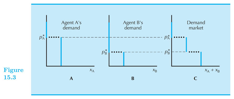
Reservation price
-
Some goods come in large discrete units
-
Reservation price is price that just makes a person indifferent
-
$ u (0 , m) = u(1, m − p^{*}_{a}) $
-
Add up demand curves to get aggregate demand curve
Market demand - discrete goods
Elasticity
Measures responsiveness of demand to price
$$ \epsilon = \frac{p}{x} \frac{dx}{dp} $$
-
What does elasticity depend on? In general, how many and how close substitutes a good has.
-
What does it mean? Why is not just the derivative?
-
We care about the magnitude so we often use: $ | \epsilon | $ instead of $ \epsilon $
Elasticity classification
-
Elastic demand: absolute value of elasticity greater than $ 1 $
-
Inelastic demand: absolute value of elasticity less than $ 1 $
Elasticity - Example for linear demand curve:
-
We will use q instead of $ x_1 $ or $ x_2 $
-
Let demand curve be: $ q = a − bp $
-
Price elasticity of demand: $ ε = −b \frac{p}{q} = \frac{−bp}{a−bp} $
Elasticity - Example for linear demand curve:

Elasticity - Iso-elastic demand curve:
Let demand curve be: $ Q = A p^{-b} $
Lets calculate the elasticity:
$$ \begin{aligned} \epsilon &= \frac{p}{Q} \frac{dQ}{dp} \\ &= \frac{p}{ A p^{-b} } ~ A (-b p^{-b-1} ) \\ &= \frac{A}{A} (-b) \frac{p ~ p^{-b-1} }{ p^{-b} } \\ &= -b \\ \end{aligned} $$
Revenue
Revenue, price increase and elasticity
Demand curve: $ Q^d = Q(p) $
Revenue: $ R = p \times Q $
When does an increase in price turn into an increase in revenue?
That is, when $ \frac{dR}{dp} > 0 $ ?
Revenue, price increase and elasticity
$$ \begin{aligned} \frac{dR}{dp} &= \frac{d(p Q(p))}{dp} \\ ~ &= p \frac{dQ}{dp} + Q(p) \\ ~ &= Q \big( \frac{p ~ dQ}{Q ~ dp} + 1 \big) \\ ~ &= Q ( \epsilon + 1 ) \\ \end{aligned} $$
So as long as $ \epsilon > -1 $, we will have that $ \frac{dR}{dp} > 0 $.
Revenue, price increase and elasticity
You can use the same math, to see that if $ \epsilon < -1 $, then $ \frac{dR}{dp} < 0 $.
Why does this matter? Consider the case of the linear demand where elasticity changes from 0 to -infinity as we increase price. Now we know that:
-
At a price level where demand is price-inelastic (which happens at low prices), an increase in price will increase revenue. And,
-
At a price level where demand is price-elastic (which happens at high prices), a decrease in price will increase revenue.
In conclusion, the price level that maximises revenue must be when the price-elasticity equals 1. The point we call unit-elasticity price level.