Firm's Decisions - Cost Minimization
Intermediate Microeconomics (Econ 100A)
Kristian López Vargas
UCSC
Cost Minimization Problem - intro idea
- The firm operates in two kinds of markets:
- Inputs/factor markets (e.g. it buys labor and capital)
- Final product market
Let's focus on optimal decisions regarding the first kind of market.
We will assume for now the firms has a target prod level $ q_0 $. (i.e. an isoquant!)
And, it aims to achieve that level of production in the best (most efficient) way possible.
let the fun begin
Cost Minimization Problem
The only decision the firm controls at this point is how much of inputs it uses.
So the most efficient way in this context refers to what is the "right" combination of (L,K) so achieve $ q_0 $.
The right combination is the one that minimize the cost of producing the given target level of output $ q_0 $.
Suppose wages are denoted by $ w $ and rental price of capital is denoted by $ r $.
So the firm wants to:
minimize: $ cost = w L + r K, \quad $ subject to: $ f(L,K) = q_0 $.
Isocost
Isocost: Combinations of input usage that cost the same (say $C):
Example: This is isocost at a cost of $100:
- $ w L + r K = 100 $
Example: This is isocost at a cost of $50 when wages = 20 and price of capital = 10:
- $ 20 L + 10 K = 50 $
Draw draw draw more examples until you dream of isocosts a little.
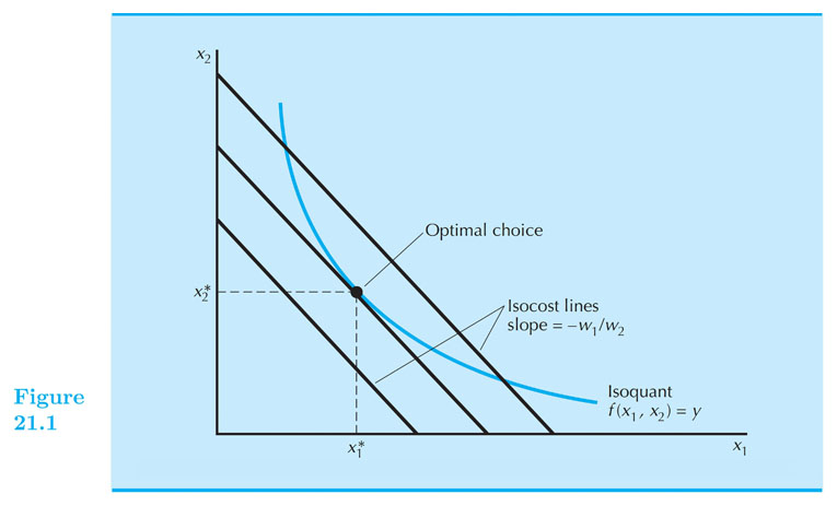
Solving the cost-minimization problem
Conceptually: find best(lowest) isocost given the required isoquant.
Graphically...
Draw the "target" output level (isoquant) $ q_0 $.
Ask: what is the cheapest combination of L,K that makes $ q_0 $ possible.
Solving the cost-minimization problem
What if prices of factors change?
What if target output changes?
Conditional factor demand functions
Optimal choices of factors are called the conditional factor demand functions
- That is: $ L^* = L(w,r,q_0) $ and $ K^* = K(w,r,q_0) $
Optimal cost is the cost function
- That is: $ c(w,r,q_0) = w L(w,r,q_0) + r K(w,r,q_0) $
Notice: all this is in the "long run" because we are able to adjust all inputs.
Cost-minimization problem - The Math
$$
\underset{L,K}{\text{minimize:}} ~ w L + r K
\\
\text{Subject to:} ~ f(L,K) = q_0
$$
Cost-minimization problem, Case 1: tangency.
If technology satisfies mainly convexity and monotonicity then (in most cases) tangency solution!
Tangency condition: slope of isoquant equals slope of isocost curve.
- In equation: $ - \frac{w}{r} = - \frac{MP_L}{MP_K} $ (EQ. 1)
Constraint: $ q = f(L,K) $ (EQ. 2)
System of two equations (Eq1 and Eq2), and two unknowns ($ L $ and $ K $).
Example: Cobb-Douglass
If $ q = f(L,K) = L K $,
$$ L^{*}(w,r,q) = \big( \frac{ q r }{ w } \big)^{1/2} $$
$$ K^{*}(w,r,q) = \big( \frac{ q w }{ r } \big)^{1/2} $$
c(w, r, q)=wL⋆ + rK⋆ = 2(qrw)1/2
Home exercise: solve the more general case:
- $ q = f(L,K) = A ~ L^{a} K^{b} $
- Find $ ~ c(w,r,q) = ?????? $
Cost-minimization problem, Case 2: Corner Solution.
Mainly, but not exclusively:
- Perfect Substitutes:
q = f(L, K)=aL + bK
- For example: $ q = f(L,K) = L + K $
Example: Linear technology (1)
q = f(L, K)=aL + bK
Compare RTS $ ( - \frac{ a }{ b }) $ Vs. slope of the isocosts $ ( - \frac{ w }{ r } ) $
Alternatively, compare: $ \frac{ a }{ w } $ Vs. $ \frac{ b }{ r } $
If $ \frac{ a }{ w } > \frac{ b }{ r } $ firm should use labor only.
If $ \frac{ a }{ w } < \frac{ b }{ r } $ firm should use capital only.
If $ \frac{ a }{ w } = \frac{ b }{ r } $ any point along the isoquant, minimizes cost.
Example: Linear technology (2)
IF $ \frac{ a }{ w } > \frac{ b }{ r } $
The firm should use only Labor (corner solution).
Then: $ q = a L $ , so $ L^*(w,r,q) = \frac{ q }{ a } $
Then: $ K^*(w,r,q) = 0 $
Then: $ c(w,r,q) = w L^\star = \frac{ w }{ a } q $
Example: Linear technology (3)
IF $ \frac{ a }{ w } < \frac{ b }{ r } $
The firm should use only Capital (corner solution).
Then: $ q = b K $ , so $ K^*(w,r,q) = \frac{ q }{ b } $
Then: $ L^*(w,r,q) = 0 $
Then: $ c(w,r,q) = r K^\star = \frac{ r }{ b } q $
IF $ \frac{ a }{ w } = \frac{ b }{ r } $, any point along the isoquant, minimizes cost.
Example: Linear technology (4)
Putting all this together:
$$ c(w,r,q)= q \times
\begin{cases}
\frac{ w }{ a },& \text{if} ~ \frac{ w }{ a } \leq \frac{ r }{ b } \\
\frac{ r }{ b },& \text{if} ~ \frac{ r }{ b } < \frac{ w }{ a }
\end{cases}
$$
This can be written as:
$$ c(w,r,q) = q ~ \textrm{min} \{ \frac{ w }{ a } , \frac{ r }{ b } \} $$
Simpler example:
If $ q = f(L,K) = L + K $, then:
c(w, r, q)=q × min{w, r}
Cost-minimization problem, Case 3: Kink Solution
- Perfect Complements (kink solution):
$$ q = f(L,K) = \text{min} \{ \frac{L}{a} , \frac{K}{b} \} $$
- if $ q = f(L,K) = \textrm{min} \{ L ,K \} $, then:
c(w, r, q)=(w + r)q
Short-run conditional demand for labor, cost function
$ K = \bar{K} $
do the graph!
Short-run conditional demand of labor: $ L = L(w,r,q, \bar{K}) $
This demand is obtained from solving L from $ q = f( \bar{K}, L) $
If there are no other inputs it does not depend on prices of inputs.
Short-run - example
$ q = f(L, K) = K^{0.5} L^{0.5} $
$ K = \bar{K} $
$ L^{SR} = \frac{ q^2 }{ \bar{K} } $
$ c^{SR}(w,r,q, \bar{K}) = w \frac{ q^2 }{ \bar{K} } + r \bar{K} $
Returns to scale and the cost function
Let us define the average cost function:
$ AC(w,r,q) = \frac{ c(w,r,q) }{ q } $
IRS implies that AC is decreasing in $ q $. (e.g. if we want to double q, we can less than double costs).
CRS implies that AC is constant in $ q $. (e.g. if we want to double q, we need to double costs).
DRS implies that AC is increasing in $ q $. (e.g. if we want to double q, we need to more than double costs).
Types of costs: Fixed and quasi-fixed costs
Fixed: costs that must be paid, regardless of output level.
Quasi-fixed cost: costs that must be paid, only if output level > 0. (heating, lighting, etc.)
Sunk cost: fixed costs that are not recoverable (painting your factory)