Consumer Choice

Intermediate Microeconomics (Econ 100 A)

Kristian López Vargas

UCSC

Consumer’s Optimal Choice

• Budget determines what I can buy.

• Utility function (preferences) determine how I value those affordable alternatives.

• Which bundle do I buy?

Consumer’s Optimal Choice

• The bundle with the highest utility among the affordable.

• We call this bundle the Rational Constrained Choice.

Three main cases of Optimal Choice.

1. Tangency Solution: When preferences are well behaved (smooth, convex, …), then at the optimal bundle: $ MRS = \frac{−p_1}{p_2} $ (for example Cobb-Douglass preferences)

2. Corner solutions or “boundary optimum”: if $ MRS > \frac{−p_1}{p_2} $ or $ MRS < \frac{−p_1}{p_2} $ always (for example: perfect substitutes)

3. Kink optimality: if preferences are “kinky” (for example: perfect complements)

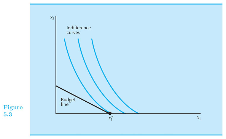
Optimal Choice - Tangency Solution

Optimal Choice - Tangency Solution (intuitively)

• Suppose your preferences look like Cobb-Douglass (smooth, convex).

• You have a BC and you are considering buying $ (x_1’, x_2’) $ such that $ x_1’>0, x_2’>0 $ on the BC.

• Suppose that only thing you know is that your MRS, at the bundle $ (x_1’, x_2’) $, is higher in magnitude than $ p_1 / p_2$. That is, the associated indifference curve is steeper than the budget constraint.

• Should you buy the bundle $ (x_1’, x_2’) $?

Optimal Choice - Tangency Solution (intuitively)

• No.

• If MRS is steeper than BC, it means that at that point you value $ x_1 $ more than the market. So…

• Buy more of that good 1.

• But how much more?

• Up to a point in which you and the market value $ x_1 $ the same (relative to $ x_2 $)

• First optimality condition: $ MRS = \frac{−p_1}{p_2} $

Optimal Choice - Tangency Solution (math method 1)

Steps to find the optimal bundle (aka the demanded bundle) for tangency cases:

1. Identify clearly the utility function.

2. Calculate the $ MRS $, it will be a function of $ x_1, x_2 $ and (possibly) on some parameters of the utility function.

3. Set the tangency condition: $ MRS = - \frac{p_1}{p_2} $ call this Equation 1.

4. Identify the budget constrain and call it Equation 2.

5. Equation 1 and Equation 2 form a 2-equation-2-unknowns system, so you can solve for the two unknowns: $ x_1 $ and $ x_2 $.

Optimal Choice - Tangency Solution (math method 1) - Example

Let’s apply these steps to the case of Cobb-Douglas preferences: $ U(x_1, x_2) = x_1^{0.5} x_2^{0.5} $

• Tangency : $ MRS = - \frac{x_2}{x_1} $. Equate MRS to: $ - \frac{p_1}{p_2} $ (Eq1)

• Budget constraint : $ p_1 x_1 + p_2 x_2 = m $ (Eq2)

• [ solve for x1 and x2 in the system of two equations – details in doc camera ]

• Optimal bundle: $ x_1^{*} = \frac{1}{2} \frac{m}{p_1} $ and $ x_2^{*} = \frac{1}{2} \frac{m}{p_2} $

Optimal Choice - Tangency Solution - Cobb-Douglas Function

• Note if you have Cobb-Douglass utility, $ U = x_1^{a} x_2^{b} $, you can always use method 1.

• Exercise: apply method 1 to this utility function: $ U = x_1^{a} x_2^{b} $

• An alternative to method 1, is a more general method called the Lagrange Method that we will cover later.

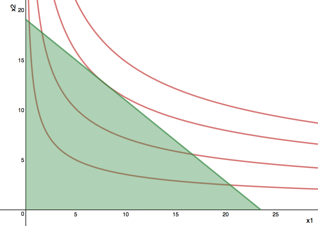
Cobb-Douglas - Typical Graph

Case 2: Optimal bundle in corner solutions

The most typical case of this type of solution is with perfect substitutes preferences.

Steps to finding the optimal bundle when x_1 and x_2 are perfect substitutes:

2. Calculate the $ MRS $, it will be a function of $ x_1, x_2 $ and (possibly) on some parameters of the utility function.

3. Compare its magnitude to the price ratio: $ \frac{p_1}{p_2} $.

4. If $ |MRS| > \frac{p_1}{p_2} $, then all income is spent on good 1: $ x_1 = m / p_1 $ and $ x_2 = 0 $

5. If $ |MRS| < \frac{p_1}{p_2} $, then all income is spent on good 2: $ x_2 = m / p_2 $ and $ x_1 = 0 $

6. If $ |MRS| = \frac{p_1}{p_2} $ any bundle that exhaust income will be optimal.

Finding the optimal bundle (perfect substitutes) - Example!

1. Say, $ u = 2 x_1 + x_2 $

2. $ MRS = - 2 / 1 = - 2 $

3. Compare |MRS| to price ratio: 2 vs. $ \frac{p_1}{p_2} $.

4. If $ \frac{p_1}{p_2} < 2 $, then: $ x_1 = m / p_1 $ and $ x_2 = 0 $

5. If $ \frac{p_1}{p_2} > 2 $, then: $ x_1 = 0 $ and $ x_2 = m / p_2 $

6. If $ \frac{p_1}{p_2} = 2 $, any $ (x_1, x_2) $ such that $ p_1 x_1 + p_2 x_2 = m $ is optimal.

Perfect substitutes

• See graphs in document camera

• See graphs on EconGraphs

Case 3: Optimal bundle in “kink” solutions

Most cases of “kink” solutions appear because of “perfect complement” preferences.

Steps to find the optimal bundle under “perfect complement” preferences:

1. Identify clearly the utility function: $ U = \textrm{min} \{ \frac{x_1}{\alpha}, \frac{x_2}{\beta} \} $, for $ \alpha, \beta > 0 $

2. Calculate the optimal consumption path: $ \frac{x_1}{\alpha} = \frac{x_2}{\beta} $. Call this Equation 1.

3. Identify the budget constraint and call it Equation 2.

4. Equation 1 and Equation 2 form a 2-equation-2-unknowns system, so you can solve for the two unknowns: $ x_1 $ and $ x_2 $.

Finding the optimal bundle - Perfect complements - Numerical Example

1. $ U = \textrm{min} \{ \frac{x_1}{2}, x_2 \} $.

2. Optimal consumption path: $ \frac{x_1}{2} = x_2 $. This is Equation 1.

3. Budget Constraint $ m = p_1 x_1 + p_2 x_2 $

4. Optimal bundle: $ x_1^{*} = \frac{m}{p_1 + p_2/2} $ and $ x_2^{*} = \frac{m}{2 p_1 + p_2} $

Perfect Complements

Optimal choice with Lagrange’s Method

• We are back to case 1 or “tangency solution”.

• Conditions:

  • Utility function is differentiable and preferences are convex,

  • $ MRS(0,y) = infinity $ and $ MRS(x,0) = 0 $

• E.g. Cobb-Douglas satisfies these conditions.

• You can always use the Lagrange’s method.

Optimal choice with Lagrange’s Method - Steps

1. Set Problem: $ \textrm{maximize} \quad U(x_1, x_2) $ subject to: $ m = p_1 x_1 + p_2 x_2 $

2. Write Lagrange’s function
   • $ L = U(x_1, x_2) - \lambda ( p_1 x_1 + p_2 x_2 - m) $
3. Differentiate with respect to $ x_1, x_2, \lambda $, equate to zero.
   • $ \frac{\partial L}{\partial x_1} = \frac{\partial U}{\partial x_1} - \lambda p_1 = 0 $
   • $ \frac{\partial L}{\partial x_2} = \frac{\partial U}{\partial x_2} - \lambda p_2 = 0 $
   • $ \frac{\partial L}{\partial \lambda} = - p_1 x_1 - p_2 x_2 + m = 0 $
   • This system of equations is called the “First Order Conditions”

4. Solve system of three equations for three unknowns (x₁, x₂, λ)

Tangency conditions from Lagrange’s method

You can obtain the “tangency condition” from using the first two conditions or equations of the Lagrangean method.

Notice that: $ \frac{\partial U}{\partial x_1} - \lambda p_1 = 0 $ can be rewritten as: $ \frac{MU_1}{p_1} = \lambda $

Similarly, $ \frac{\partial U}{\partial x_2} - \lambda p_2 = 0 $ can be rewritten as: $ \frac{MU_2}{p_2} = \lambda $

Therefore we can equate those to and obtain: $ \frac{MU_1}{p_1} = \frac{MU_2}{p_2} $

…which can be rewritten as: $ \frac{MU_1}{MU_2} = \frac{p_1}{p_2} $

which is nothing but the tangency condition.

More in general…

In general, the Lagrangean method gives you $ n+1 $ equations, where n is the number of goods in the utility function.

The first n equations are $ \frac{\partial L}{\partial x_i} = 0 $ for $ i = 1, …, n$.

The last equation, $ \frac{\partial L}{\partial \lambda} = 0 $, boils down to the budget line, always.

With the n + 1 we need to find the solution for the n expressions for $ x_1, …, x_n $ and for $ $.

Optimal choice with Lagrange’s Method - Example

0. Consider: $ \quad U(x_1, x_2) = x_1^{0.5} + x_2^{0.5} $

1. Problem: $ \quad \textrm{maximize} \quad x_1^{0.5} + x_2^{0.5} $ subject to: $ m = p_1 x_1 + p_2 x_2 $

2. Lagrange’s function: $ \quad L = x_1^{0.5} + x_2^{0.5} - \lambda ( p_1 x_1 + p_2 x_2 - m) $

3. Differentiate with respect to $ x_1, x_2, \lambda $, equate to zero.
   • $ \frac{\partial L}{\partial x_1} = 0.5 x_1^{-0.5} - \lambda p_1 = 0 $
   • $ \frac{\partial L}{\partial x_2} = 0.5 x_2^{-0.5} - \lambda p_2 = 0 $
   • $ \frac{\partial L}{\partial \lambda} = - p_1 x_1 - p_2 x_2 + m = 0 $

4. Solution good 1: $ \quad x_1^* = \frac{ m }{ p_1 + p_2 } \frac{ p_2 }{ p_1 } $

5. Solution good 2: $ \quad x_2^* = \frac{ m }{ p_1 + p_2 } \frac{ p_1 }{ p_2 } $

Practice all these cases with the lagrange’s Method.

1. $ U(x_1, x_2) = x_1^{1/2} x_2^{1/2} $

2. $ U(x_1, x_2) = x_1^{1/4} x_2^{3/4} $

3. => $ U(x_1, x_2) = x_1^{a} x_2^{b} $

4. $ U(x_1, x_2) = x_1^{a} x_2^{1-a} $

5. $ U(x_1, x_2) = (1/4) ln(x_1) + (3/4) ln(x_2) $

6. $ U(x_1, x_2) = a x_1 + b ln(x_2) $

Tangency does not work with non-convex preferences

• Be careful with tangency conditions.

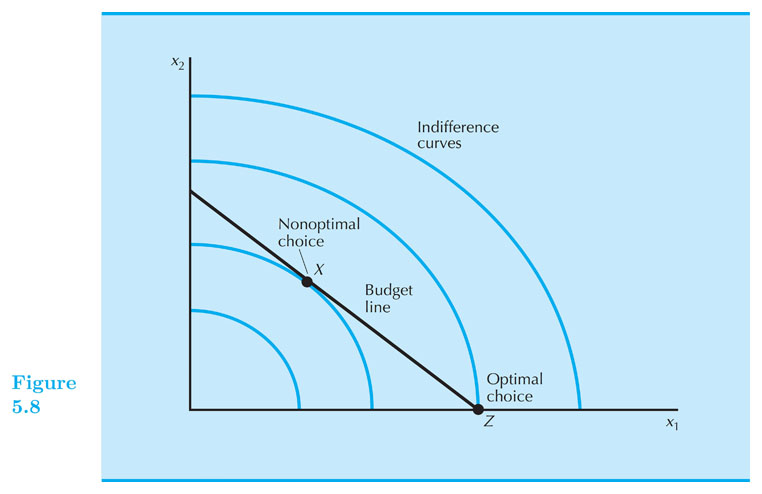
Corner solutions are not only for perfect substitutes

All cases (with examples) EconGrahps