Firm Supply and Industry Supply

Intermediate Microeconomics (Econ 100A)

Kristian López Vargas

UCSC

Recap on concepts and notation

Remember that we can write marginal cost in three different ways:

$ \frac{∂ c(q) }{ ∂q} = c'(q) = MC(q) $ where $ c(y) $ is the cost function.

Remember that revenue or "sales" are given by:

$ R(q) = p \times q $

Firm's constraints:

• Technological constraints: what can be produced, how and from what inputs

  • The shape of the cost function if determined by production function and prices of inputs.

• Market constraints: how will consumers and other firms react to a given firm’s choice?

  • If I charge high price, I cannot sell many units.

Perfect competition

Key feature of perfect competition: agents take market price as given, outside of any particular firm’s control.

This happen, typically, when many small agents operate in either side of the market.

If the firm is a price-taker at price level $ p^* $ (e.g. the firm is one of many many producers) and tries to sell for a higher price, then it will sell zero units.

If the firm charges exactly $ p^* $, it can produce/sell pretty much as much as it wants. BUT What is the right quantity??

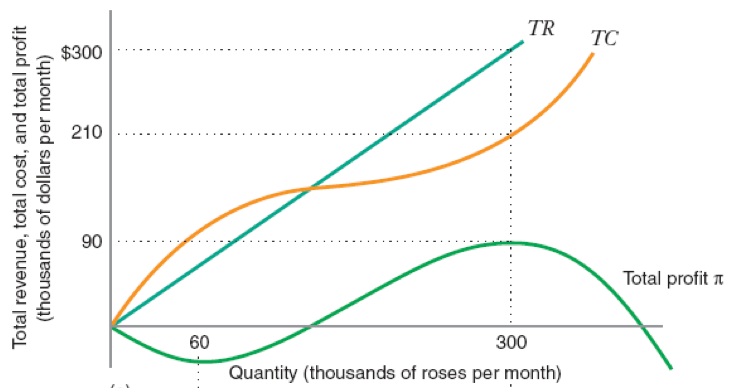
Total Revenue, Total Cost, and Profit

Supply function of a competitive firm

We assume the firm wants to maximize profits $ \pi(q) = p \times q − c(q) $

If $ \pi(q) $ is smooth and has a global maximum, the optimal $ q $ is found by setting:

$$ \frac{∂ \pi(q) }{ ∂q} = 0 $$

As before, we call this the first-order condition (FOC).

Supply function of a competitive firm

The first-order condition (FOC) implies:

$$ \begin{aligned} \frac{∂ \pi(q) }{ ∂q} &= 0 \\\\ MR - MC(q) &= 0 \\\\ p - MC(q) &= 0 \\\\ p &= MC(q) \\\\ \end{aligned} $$

The firm's MC curve determines the firm's supply function.

Supply function of a competitive firm

However, the first order condition is not sufficient: sometimes it identifies a local minimum.

The derivative of profit wrt q is zero also at the bottom of a "valley".

While a local maximum (what we want) is found at the peak of the "hill".

How do we distinguish bottom of the valley from top of the hill?

See graph.

Supply function of a competitive firm

In the top of the hill slope goes from positive to negative, decreases.

Second-order condition: $ \pi''(q) = -c''(q) \leq 0 ~ $ or $ ~ c''(q) \geq 0 $

$$ \frac{∂ MC(q) }{ ∂q} \geq 0 $$

The supply function is not the whole MC(q), but only the segment that is upward-sloping.

Still, not the end of the story...

When does the firm indeed operate?

Compare profit from operation (q*>0) Vs. shutting down (q=0)

That is: $ p q − c_v(q) − F ~ $ Vs. $ −F $

Operate if: $ ~ p q − c_v(q) − F \geq (−F) $

That is, if: $ p q − c_v(q) \geq 0 $

That is, if: $ p \geq \frac{c_v(q)}{q} = AVC(q) $

Operate when price covers average variable cost (AVC)

Supply curve for the firm -- Finally!

Supply curve is the upward-sloping part of MC curve that also lies above the AVC curve.

Notice $ q^* = 0 $ if $ MC < minAVC $.

Identifying profits graphically

Inverse Supply curve

The inverse supply curve is the same equation of the supply curve except we have solved for p:

Mathematically:

$ p = c’(q) $

if $ c''(q) >0 $ and $ c'(q)>AVC $

Supply curve - Example - Steps

Suppose $ c(q) = q^2 +1 $

1. Calculate MC: MC = 2 q

2. Equate MC = P: $ p = 2 q $. This gives the (inverse) supply curve.

3. Make sure $ MC \geq AVC $: In this example, for any value of $ q>0 $ we have that MC > AVC, since: $ 2 q \geq q $

4. Supply is $ q = p/2 $ and inverse supply is $ p = 2q $

Short-run industry supply

The supply curve in the "short run of the industry" is the sum of the supplies of all participating firms.

$ S(p) = \sum_1^n q^s_i(p) $