2 Consumer Choice

This section presents some standard economic models of consumer behavior.

2.1 Rational Choice

The basic model of consumer choice studies the decision of a single person regarding what goods to acquire, and how much to buy of each of them, taking as given the prices of the goods and the income level of the consumer. This simple model assumes that each consumer chooses the “best” combination of goods (or bundle) that he “can afford”. The idea of “best” builds on the notions of preferences and utility; our model captures “affordability” via budget sets.

To fix ideas, suppose a person goes to the supermarket with $100. While there, he can see all the goods that are offered and their corresponding prices. The consumer problem addresses the question of how to allocate the $100 among the different goods. Its solution claims that, among all possible allocations, the person will select the one that makes him as happy as possible.

The problem of the consumer has two main components:

Preferences: The preferences of a person consist of his personal ranking over all possible alternatives. We often capture these preferences by the so called utility function.

Budget set: The budget set of an individual is the collection of all alternatives that he can afford given his resources (income or wealth) and the prices of the goods that the person faces in the market.

Under the maximization assumption, preferences and budget sets induce choices. As prices and/or income change, so does the budget set and (often) the combination of goods that the consumer selects. The demand function describes the consumption decisions for all different combinations of prices and income levels.

To simplify the exposition, we focus on a simple version of the consumer problem. The main parts of the model are as follows:

There are only two goods, good 1 and good 2. We represent the quantities of these goods as $x_1$ and $x_2$, respectively. The ordered pair $(x_1,x_2)$ denotes a bundle of goods.
The prices of goods 1 and 2 are represented by $p_1$ and $p_2$, respectively.
The income level of the consumer is denoted by $m$.

Example: Suppose good 1 is orange juice and good 2 is salad. Then $x_1$ indicates the quantity of orange juice (say in liters) and $x_2$ is the quantity of salads (say in pounds). In this context, the combination (1/2, 1) represents the bundle of half liter of orange juice and one pound of salad. Suppose also that a liter of orange juice costs $5, a pound of salad costs $10, and the income level of the consumer is $500. In our notation, this information is concisely written as $p_1$ = 5, $p_2$ = 10, and $m$ = 500. ■

This two-goods model can be easily extended to more goods (e.g., it can be extended to the set of all goods that can be found in the supermarket). We use the two-goods case because it helps us to illustrate the main concepts and tools in a simple way, often using a picture.

Budget Set

The budget set is the set of all bundles (or combinations of goods) that are affordable by the consumer. That is, the set of all $(x_1,x_2)$ that satisfy

\[p_1x_1 + p_2x_2 \leq m\]

where $p_1$, $p_2$ represent the prices of goods 1 and 2, respectively, and $m$ is his income level.

The set of bundles that exhaust the income of the consumer is called the budget line. It is given by the pairs of good quantities that satisfy

$p_1x_1 + p_2x_2 = m$.

In both cases, we also assume $x_1 \geq 0$ and $x_2 \geq 0$.

In a graph where $x_1$ is represented along the horizontal axis, and $x_2$ along the vertical axis, the intersection of the budget line with the horizontal axis is $m/p_1$. This is the amount the consumer can get of good 1 if he allocates all his income on the first good. Similarly, the intersection of the budget line with the vertical axis is $m/p_2$. This is the amount the consumer can get of good 2 if he allocates all his income on the second good. The slope of the budget line is given by $-p_1/p_2$.

The next picture shows the budget set and line for the case of $p_1 = 2$, $p_2 = 2$ and $m = 40$.

Budget Set and Budget Line

Example : Suppose the government imposes a per unit tax of $t$ dollars on good 2. Then, the new budget line is

\[p_1x_1 + (p_2 + t)x_2 = m\]

Notice that the tax reduces the number of units the consumer can afford of both goods 1 and 2. This happens even while the tax only affects the price of good 2. ■

Utility Function

Consumer preferences capture a ranking over the different combinations of goods (or bundles). For instance, if the consumer strictly prefers bundle $(x_1^{'},x_2^{'})$ = (1 pizza, 2 burritos) over bundle $(x_1^{'},x_2^{'})$ = (2 pizzas, 1 burrito), then the first combination of goods is ranked before the second one in the preferences of this consumer.

There are two important assumptions that we often impose on preferences. Firstly, we assume consumer preferences are complete. Completeness means that the consumer can always compare any pair of budles and let us know which one he prefers the most. He can also tells us that he is indifferent between the two of them. In summary, completeness only rules us the possibility that the consumer tells us he “does not know” which combination of goods he prefers.

Secondly, we assume consumer preferences are transitive. Transitivity means that if a consumer prefers bundle $a$ over bundle $b$, and he also prefers bundle $b$ over bundle $c$, then it must be the case that the consumer prefers bundle $a$ over bundle $c$. Transitivity is a very important property as it allows us to talk of the most preferred bundle!

Only when these two assumptions hold, we can (often) conveniently represent the preferences of a given consumer by what we call a utility function¹.

Formally, a utility function is a function that assigns a number to each bundle in such a way that these numbers respect the underlying preference ranking of the consumer (i.e., the utility function assigns higher numbers to more preferred combinations of goods).

Example : Let good 1 be pizza and good 2 be burrito. In addition, assume the preferences of a given consumer over slices of pizza and burritos are captured by the next utility function:

\[u(x_1,x_2) = (x_1)^{1/4} (x_2)^{3/4}\]

Suppose that a first bundle contains 16 slices of pizza and 1 burrito, so that $u(16,1)=2$. If a second bundle has 3 slices of pizzas and 3 burritos, then $u(3,3)=3$. It follows that this consumer prefers the second over the first combination of goods (i.e., he likes to have 3 slices of pizzas and 3 burritos more than having 16 slices of pizza and 1 burrito). ■

Though there are many types of utility functions, three of them are of particular importance: Cobb-Douglas, Perfect Complements (i.e., Leontieff), and Perfect Substitutes (i.e., linear). We will sometimes also use the CES utility function. (CES stands for constant elasticity of substitution. We will clarify this term later.) The specific mathematical (functional) form of each of these utilities is given in the next table.

Utility Function	Mathematical Form
Perfect Substitutes	$u(x_1,x_2) = ax_1 + bx_2$
Perfect Complements	$u(x_1,x_2) = min\{ \frac{x_1}{a} , \frac{x_2}{b} \}$
Cobb-Douglas	$u(x_1,x_2) = (x_1)^a (x_2)^b$
CES	$u(x_1,x_2) = (ax_1^r + bx_2^r)^{1/r}$

In the first three cases we typically assume $a,b \ge 0$. In the last one, we let $r \leq 1$. As we shall see, these parameters play very different roles in each specification.

As we explained earlier, the important aspect of a utility function is that it captures the underlying preferences of a specific consumer. According to the ordinal utility theory, it is meaningful to ask whether a bundle is better than a second one, but not how much better it is. In other words, the actual numbers that a utility function assigns to the specific bundles are not important as far as they preserve (respect) the ranking of the individual over the combination of goods. It follows that when the preferences of an individual can be represented by a utility function, then an infinite number of them can capture the same preferences!

Example : Suppose that our previous consumer strictly prefers 16 slices of pizza and 1 burrito to 3 slices of pizzas and 3 burritos. In addition, he is indifferent between having 3 slices of pizzas and 3 burritos and 2 slices of pizzas and 4 burritos. Moreover, he strictly prefers 2 slices of pizzas and 4 burritos to having 2 slices of pizzas and 2 burritos. In summary, this consumer ranks the different combinations of goods as follows:

\[1^{st} \; (16,1); \quad 2^{nd} \;(3,3) \; and \; (2,4); \quad 3^{rd}\; (2,2)\]

It follows that a utility function represents his preferences if and only if it assigns numbers to each combination of goods in the following way:

\[u(16,1) > u(3,3)=u(2,4) > u(2,2)\]

Let us now consider the three possible utility functions shown in the next table. Which of these three utilities represent the preferences we just described?

Bundle	Utility 1	Utility 2	Utility 3
$(16,1)$	8	12	4
$(3,3)$	7	9	2
$(2,4)$	6	9	2
$(2,2)$	3	2	-1

It is clear that Utility 1 does not do so. The reason is that it assigns to bundle $(3,3)$ a higher number than to bundle $(2,4)$, contradicting the fact that the consumer is indifferent between these two combinations of goods. On the other hand, even when Utility 2 and Utility 3 assign different numbers to the bundles, both of them are consistent with the preference ranking of the consumer. Therefore, Utility 2 and Utility 3 both represent this consumer’s preferences. ■

There are two concepts associated with the utility function, which play a key role in explaining consumer behavior, namely, indifference curves and marginal rate of substitution. We describe each of them next.

An indifference curve is the set of all bundles that a consumer regards as equally desirable. In other words, it is the set of all combinations of goods that give the consumer the same utility level.

We often assume that preferences satisfy a property that says more is always better. Under this monotonicity assumption, the indifference curves cannot be “thick” and they must be downward sloping.

Weakly preferred sets also provide a convenient characterization of preferences. In terms of the utility function, a weakly preferred set is the sets of all bundles $(x_1,x_2)$ such that $u(x_1,x_2)$ is at least as large as a specific value $k$.

Example : Let $u(x_1,x_2) = (x_1)^{1/4} (x_2)^{3/4}$. Then,

\[u(x_1,x_2) = (x_1)^{1/4} (x_2)^{3/4} = k\]

implicitly describes the set of all combinations of goods 1 and 2 that give the consumer a level k of utility. For each k, this set —which can be also written as $x_2 = \frac{k^2}{x_1}$— denotes a specific indifferent curve. We can get all the indifference curves by changing $k$.

In addition, for each $k$, the associated weakly preferred set is $x_2\geq \frac{k^{4/3}}{x_1^{1/3}}$. ■

The next figure shows the typical shape of the indifference curves for the case of Perfect Substitutes (top, left), Perfect Complements (top, right), Cobb-Douglas (bottom, left) and CES (bottom, right). You can find an interactive version of this figure here.

(a) Perfect Substitutes

b) Perfect Complements

(d) CES

As we will explain, the marginal rate of substitution (MRS) is intimately related with the concept of marginal utility (MU). Thus, we start describing the latter.

The marginal utility of good 1 captures the extra utility the consumer gets if he slightly increases the consumption of good 1, while keeping fixed the consumption of the second good. We can similarly define the marginal utility of good 2. When the utility function $u(x_1,x_2)$ is differentiable, then the marginal utilities of goods 1 and 2, denoted by $MU_1$ and $MU_2$, are simply the partial derivatives of $u(x_1,x_2)$ with respect to goods 1 and 2, respectively. That is,

\[MU_1 = \frac{\partial u(x_1,x_2)}{\partial x_1} \quad and \quad MU_2 = \frac{\partial u(x_1,x_2)}{\partial x_2}\]

Example : Let $u(x_1,x_2) = (x_1)^{1/4} (x_2)^{3/4}$. Then,

$MU_1 (x_1,x_2) =\frac{1}{4}(x_1)^{-3/4} (x_2)^{3/4} \quad and \quad MU_2 (x_1,x_2) =\frac{3}{4}(x_1)^{1/4} (x_2)^{-1/4}$ ■

We showed before that two different utility functions might induce the same ranking over consumption bundles. These two utility functions represent the same preferences. As the next example illustrates, an issue with the concept of marginal utility is that it is sensitive to the way in which we represent consumer preferences.

Example : Let us work with the same utility as in the previous example, $u(x_1,x_2) = (x_1)^{1/4} (x_2)^{3/4}$, except that now we multiply it by 4. That is, $u(x_1,x_2)= 4(x_1)^{1/4}(x_2)^{3/4}$. Then,

\[MU_1 (x_1,x_2) =(x_1)^{-3/4} (x_2)^{3/4} \quad and \quad MU_2 (x_1,x_2) =3(x_1)^{1/4} (x_2)^{-1/4}\]

Since this utility is just $u(x_1,x_2)=(x_1)^{1/4} (x_2)^{3/4}$ multiplied by 4, it represents the same ranking over consumption bundles as the utility of the previous example. Nevertheless, the two MUs are four times as large with $u(x_1,x_2)=4(x_1)^{1/4} (x_2)^{3/4}$ as compared to $u(x_1,x_2)=(x_1)^{1/4} (x_2)^{3/4}$ ■

Notice that the utility function is monotone increasing in the two goods (i.e., more is always better!) then the MUs are always positive.

As we mentioned above, a second concept related to the utility function that is very important in economics is the marginal rate of substitution (MRS). The MRS is a measure of the relative value of good 1 in terms of good 2. In particular, it measures (approximately) how much the consumer is willing to give up of good 2 in order to obtain an additional unit of good 1.

Mathematically, the MRS is given by the slope of an indifference curve (IC) at a given bundle. Therefore, it can be obtained as follows: Assuming that preferences are monotonic and can be represented by the utility function $u(x_1,x_2)$, we can think of an IC as a function $x_2(x_1)$. Along this IC, we have:

\[u(x_1,x_2(x_1))= k\]

If we differentiate this function with respect to $x_1$ (using the Chain Rule), we get:

\[\frac{\partial u}{\partial x_1}(x_1,x_2) + \left[ \frac{\partial u}{\partial x_2} (x_1,x_2)\right] \frac{\partial x_2}{\partial x_1}(x_1) = 0.\]

Since the MRS is the slope of the IC, we get that

\[MRS = \frac{\partial x_2}{\partial x_1}(x_1) = \frac{-MU_1}{MU_2}.\]

A very important property of the MRS is that (unlike the marginal utilities MUs) it is not affected by the way in which we measure preferences!

Example : Let the utility function be either $u(x_1,x_2) = (x_1)^{1/4} (x_2)^{3/4}$ or $u(x_1,x_2)= 4(x_1)^{1/4}(x_2)^{3/4}$. In both cases, we have that

\[MRS(x_1, x_2) = \frac{-MU_1 (x_1,x_2) }{MU_2 (x_1,x_2)} = \frac{-x_2}{3x_1}\]

In other words, the MRS remains the same for both utilities. ■

When the utility function increases in the consumption of each good, then the MRS is negative. This means that if the consumer sacrifices a bit of one good, then he must be compensated with a bit more of the other good to be as well as before.

In addition, we often assume that the MRS is decreasing (in absolute value). This captures the idea that the consumer prefers some sort of diversification across goods —he prefers to have some of each good rather than having a lot of one good and nothing of the other. A decreasing MRS means that the more the consumer sacrifices one good, the more he needs to be compensated with the other one to be as well as before. When this happens, we say that consumer preferences are convex.

Optimal Choice

We have discussed both consumer’s preferences (captured by his utility function) and consumption restrictions (captured by his budget set). To characterize consumer behavior —that is, to explain the bundle that he will acquire in the market for each combination of prices and income level— we assume the consumer behaves in an optimal way. In words, we postulate that the consumer selects the most desirable bundle out of the ones that he can actually afford.

Mathematically, this implies that the consumer solves the following problem:

\[max_{x_1,x_2} \; \{u(x_1,x_2): p_1x_1+p_2x_2=m\}\]

We start with a graphical explanation for the solution of the consumer problem.

The next figure shows the case of a consumer with income level $m=40$, who faces prices $p_1=2$ and $p_2=2$. Thus, his budget set is $2x_1+2x_2 \leq 40$, which is illustrated in the shaded triangular area. Suppose that the utility function of this consumer has a Cobb-Douglas specification $u(x_1,x_2)=x_1^{3/4}x_2^{1/4}$. The figure also shows four ICs corresponding to the following different utility levels: $k_1=6$, $k_2=9$, $k_3=11.39$, and $k_4=15$. As it is readily verified, the further away from the origin, the higher the utility level of the consumer.² Recall that we assume the consumer acquires the most desirable combination of goods among the ones that he can afford. This consumer can definitely get a utility level of 6 —since there are some affordable bundles (under the shaded area) that provide this level of satisfaction. The same applies to a utility of level of 9. Notice that this is not true for a utility of level 15 —since there is no affordable bundle that provides the consumer this level of satisfaction. It turns out that, in this example, the highest achievable utility level is $k_3=5^{1/4}15^{3/4}= 11.39$, with the optimal consumption bundle being $(5,15)$.

It follows from our simple example that the best affordable combination of goods is the one that belongs to the highest IC that just touches —usually in only one point— the budget constraint.

Graphical solution to the consumer problem

Note: For an interactive version of this graph visit: https://www.desmos.com/calculator/v9m2vj24vx

We now present the mathematical solution of the consumer problem for three of the most commonly used utility functions.

Optimal Choice With Cobb-Douglas Preferences

The consumer problem with Cobb-Douglas preferences is given by

\[max_{x_1,x_2} \; \{x_1^a x_2^b: p_1x_1+p_2x_2=m\}\]

To find the optimal bundle when preferences are Cobb-Douglas (C-D), we use the Lagrangian method. The associated Lagrangian function is

\[L(x_1,x_2,\lambda)=x_1^a x_2^b-\lambda(p_1x_1+p_2x_2 - m)\]

Recall that we can get the solution of our initial problem by finding the maximizers of the Lagrangian function. The first order conditions of our problem (FOCs) are:

$\partial L / \partial x_1= ax_1^{a-1} x_2^b -\lambda p_1 = 0$ (FOC1)
$\partial L / \partial x_2= bx_1^a x_2^{b-1} -\lambda p_2 = 0$ (FOC2)
$\partial L / \partial \lambda = -p_1x_1-p_2x_2+m = 0$ (FOC3)

To find the optimal consumption bundle, we need to find the $x_1$, $x_2$, and $\lambda$ that solve this system of three equations and three unknowns (as a function of $p_1$, $p_2$ and $m$).

We can solve this system of equations by finding a conection between $x_1$ and $x_2$ via FOC1 and FOC2. In particular, FOC1 and FOC2 can be re-written as

\[\frac{ax_1^{a-1} x_2^b}{p_1} = \lambda \quad and \quad \frac{bx_1^a x_2^{b-1}}{p_2} = \lambda\]

Making these two terms equal to each other we get:

\[\frac{ax_1^{a-1} x_2^b}{p_1} = \frac{bx_1^a x_2^{b-1}}{p_2}\]

This expression simplifies to:

\[\frac{ax_2}{bx_1} = \frac{p_1}{p_2}\]

Combining this last result with FOC3, we finally get:

\[x_1^* = \frac{a}{a+b}\frac{m}{p_1} \quad\quad x_2^* = \frac{b}{a+b}\frac{m}{p_2}\]

(To find $\lambda^*$, we can simply plug $x_1^*$ and $x_2^*$ into either FOC1 or FOC2, though we are usually not interesting in the value of this variable.)

It follows from our previous results, that the optimal solution satisfies

\[MRS = \frac{p_1}{p_2} \quad and \quad m = p_1x_1 + p_2x_2.\]

The first condition states that the relative value of the goods from the perspective of the consumer has to equal their relative value from the perspective of the market. The second condition simply states that the optimal bundle must be on the budget line.

Example : Let us assume that $u(x_1,x_2) = x_1^a x_2^b$ with $a = ¼$, $b = ¾$, $m = 40$, $p_1 = 2$ and $p_2 = 2$. Thus, the Lagrangian of the problem is:

\[L(x_1,x_2,\lambda)=x_1^{1/4}x_2^{3/4} -\lambda(2x_1+2x_2-40)\]

Taking the partial derivatives with respect to $x_1, x_2$ and $\lambda$, we get:

$\partial L / \partial x_1= (1/4)x_1^{1/4-1} x_2^{3/4} -\lambda 2 = 0$ (FOC1)
$\partial L / \partial x_2= (3/4)x_2^{3/4} x_1^{1/4-1} -\lambda 2 = 0$ (FOC2)
$\partial L / \partial \lambda = 40-2x_1-2x_2 = 0$ (FOC3)

To find the optimal $x_1$ and $x_2$, we first get from FOC1 and FOC2 and then make these two terms equal to each other:

\[\frac{1/4 x_1^{-3/4} x_2^{3/4}}{2} = \frac{3/4 x_2^{-1/4} x_1^{1/4}}{2}\]

This expression simplifies to:

\[\frac{x_2}{3x_1} = \frac{p_1}{p_2}\]

Combining the latter with FOC3, we solve for $x_1$ and $x_2$ and obtain:

$x_1^* = \frac{1}{4} * \frac{40}{2} = 5 \quad and \quad x_2^* = \frac{3}{4} * \frac{40}{2} = 15$ ■

Optimal Choice With Perfect Substitutes Preferences

When the goods are perfect substitutes from the perspective of the consumer, then we cannot use the Lagrangian method to obtain the optimal bundle. The reason is that, in this case, the solution is usually non-interior. We next explain how to approach the consumer problem in this case.

The consumer problem with perfect substitute preferences is given by:

\[max_{x_1,x_2} \; \{ax_1+bx_2: p_1x_1+p_2x_2=m\}\]

In this case, the MRS (in absolute value) between the goods is given by:

\[MRS = a/b\]

Recall that the MRS defines the relative value of good 1 in terms of good 2 from the perspective of the consumer. With perfect substitute preferences, the MRS is just a constant.

On the other hand, the ratio $p_1/p_2$ describes the relative market valuation of good 1 in terms of good 2.

In the case of perfect substitutes, the optimal choice relies on the comparison between the MRS and the ratio of prices.

Case 1: If $MRS = a/b > p_1/p_2$ then $x_1^* = m/p_1$ and $x_2^* = 0$

Case 2: If $MRS = a/b < p_1/p_2$ then $x_1^* = 0$ and $x_2^* = m/p_2$

Case 3: If $MRS = a/b = p_1/p_2$ then $x_1^* \in [0,m/p_1]$ and $x_2^* \in [0,m/p_2]$ such that $p_1x_1^*+p_2x_2^*=m$

To understand the first case, notice that $a/b > p_1/p_2$ means that the extra value of the first good as compared to the second one from the perspective of the consumer is higher than the extra cost of getting the first good as compared to getting the second one. Thus, it is convenient for this person to spend all his income in the first good. Case 2 has a similar explanation. Case 3 corresponds to a situation in which the MRS equals the relative prices; in this last case, the consumer is indifferent between spending all, some, or no money in good 1 as far as he spends the rest of his income in the other good

Example : Suppose $a = 1.5$ and $b = 1$. Then, $MRS = 1.5$. This means that this consumer is willing to give up to 1.5 units of good 2 for an additional unit of good 1. On the other hand, let us assume that $p_1=2, p_2=2$ and $m=40$. Thus, the relative market value of good 1 in terms of good 2 is just 1, i.e., $p_1/p_2=1$. Given that

\[MRS = 1.5 > 1 = p_1 / p_2\]

regardless of the bundle selected, we are in Case 1 above. Thus, it is optimal for the consumer to spend all his income in good 1. That is,

\[x_1^* = \frac{m}{p_1} = \frac{40}{2} = 20 \quad\quad x_2^* = 0\]

The next figure illustrates this solution. ■

Solution for the perfect substitutes

Optimal Choice with Perfect Complement Preferences

Remember that the utility function for perfect complement preferences is given by

\[u(x_1,x_2) = min\{\frac{x_1}{a},\frac{x_2}{b}\}\]

As with the case of perfect substitutes, when the goods are perfect complements from the perspective of the consumer, then we cannot use the Lagrangian method to obtain the optimal bundle. In this case, the reason is that the corresponding utility function is not differentiable.

The consumer problem with perfect complements utility function is given by

\[max_{x_1,x_2}\{min\{\frac{x_1}{a},\frac{x_2}{b}\}:\quad p_1x_1+ p_2x_2 =m \}\]

Notice that, in this case, as long as p1, p2, a and b are all strictly positive, the optimal bundle will always satisfy:

\[\frac{x_1}{a} = \frac{x_2}{b}\]

The reason is quite simple. Suppose that instead we have $x_2/b > x_1/a$ . Then,

\[x_2/b>x_1/a = u(x_1,x_2)=min\{x_1/a , x_2/b\}\]

It follows that this consumer could be strictly better off by spending a bit less in the second good and using that money to get a bit more of the first good! This process repeats till $x_1/a = x_2/b$. (A similar idea applies when $x_1/a > x_2/b$.)

In addition, we know that the optimal bundle must satisfy the budget constraint. That is,

\[p_1x_1 + p_2x_2 = m\]

Combining our two observations, we get:

\[p_1x_1 + p_2 \frac{bx_1}{a} = m\]

so that $x_1^* = \frac{ma}{(ap_1 + bp_2)}$. In a similar way, we get that $x_2^* = \frac{mb}{(ap_1 + bp_2)}$

Example : Let us assume $u(x_1,x_2)= min\{ \frac{x_1}{a},\frac{x_2}{b}\}$ with $a=1$, $b=1$, $p_1=2$, $p_2=2$, and $m=40$. In this case, we know that the optimal consumption of good 1 and 2 must satisfy:

\[x_1=x_2\]

We also know that:

\[2x_1 + 2x_2 = 40\]

Using these two equations, we get that:

\[x_1^* = \frac{ma}{(ap_1 + bp_2)} = \frac{40}{2+2} = 10 \quad x_2^* = \frac{mb}{(ap_1 + bp_2)} = \frac{40}{2+2} = 10\]

The next figure illustrates this solution. ■

Solution for the perfect complements

2.2 Demand Function

Individual Demand Function

We explained earlier that the consumer problem consists of selecting the most preferred bundle among the ones that the consumer can afford. Mathematically, the problem was described as follows:

\[max_{x_1,x_2} \; \{u(x_1,x_2): p_1x_1+p_2x_2=m\}\]

The solution of this problem is a pair $x_1^*$ and $x_2^*$. We typically write this choice as:

\[x_1^* = x_1(p_1,p_2,m) \quad and \quad x_2^* = x_2(p_1,p_2,m)\]

to highlight the fact that the optimal amounts of good 1 and good 2 depend on the prices of the goods and the income level of the consumer. In other words, optimal choices are function of $p_1, p_2$ and $m$ . We refer to these functions as the individual demand functions.

The demand function of good $i$ (with $i=1,2$) receives different names according to the way in which it responds to changes in each of its arguments. (In economics, we often call this exercise comparative statics.) We next describe the main relationships.

Changes with respect to income:

If $x_i(p_1,p_2,m)$ increases with $m$, we say the good is normal.
If $x_i(p_1,p_2,m)$ decreases with $m$, we say the good is inferior.

Changes with respect to own price:

If $x_i(p_1,p_2,m)$ decreases with $p_i$, we say the good is ordinary.
If $x_i(p_1,p_2,m)$ increases with $p_i$, we say the good is Giffen.

Changes with respect to the price of the other good:

If $x_i(p_1,p_2,m)$ increases with $p_j$, we say the good is substitutes.
If $x_i(p_1,p_2,m)$ decreases with $p_j$, we say the good is complements.

Out of all these possibilities, Giffen goods are probably the less frequently observed. Jensen and Miller (AER, 2008) provided the first real-world evidence of Giffen behavior, i.e., a good with upward-sloping demand. The authors found this behavior when studying rice subsidies for poor households in Hunan and Gansu, China.

The next example shows the effects of prices and income on the demand function generated by a Cobb-Douglass utility function.

Example : Let the utility be $u(x_1,x_2) = x_1^{1/4} x_2^{3/4}$. We showed before that, in this case,

\[x_1^* = x_1 (p_1,p_2,m) = \frac{1}{4}\frac{m}{p_1} \quad and \quad x_2^* = x_2 (p_1,p_2,m) = \frac{3}{4}\frac{m}{p_2}\]

Thus, according to our previous definitions, both goods are normal and ordinary. Since the quantity demanded of one of them does not depend on the price of the other one, we also say that they are independent. ■

The next figures provide a graphical representation of our comparative statics results.

Own price changes:

Optimal choice at different $p_1$ levels

Demand curve

Income Changes:

Optimal choice at different income levels

Testable Implications of the Model

Our previous classifications of the goods seem to suggest that about any change in consumption is possible as prices and income levels change. Thus, one immediately wonders:

\[Does \; our \; theory \; generate \; any \; testable \; implication?\]

We will show that the answer is yes. This is important as, otherwise, our theory of consumer choice could never be proven false!

The testable implication of our theory receives the name of Weak Axiom of Revealed Preferences (WARP). This basic result is quite simple. If a bundle is acquired, then it must be the case that the consumer prefers this combination of goods to any other affordable one. In other words, via choices, the consumer is providing us some information regarding his preferences. By testing WARP we make sure that consumer’s choices don’t provide contradicting information. The next example illustrates this possibility.

Example : Imagine that we observe the next choices.

Price of good 1	Price of good 2	Income	Choice of good 1	Choice of good 2
$p_1$ = 2	$p_2 = 1$	$m=10$	$x_1^* = 4$	$x_2^* = 2$
$p_1$ = 1	$p_2 = 1$	$m=8$	$x_1^* = 1$	$x_2^* = 7$

We are interested in the next question:

\[Could \; these \; choices \; have \; been \; made \; by \; a \; utility \; maximizer?\]

The answer is no. The reason is as we describe next.

When the prices and income level were given by $p_1=2, p_2=1,$ and $m=10$, the consumer selected 4 units of good 1 and 2 units of good 2. Notice that, since $2*1+17<10$, he could have selected to consume 1 unit of good 1 and 7 units of good 2. This is telling us that this consumer strictly prefers bundle (4, 2) to bundle (1, 7).

Alternatively, when the prices and income level of the consumer were given by $p_1=1, p_2=1,$ and $m=8$, he selected 1 unit of good 1 and 7 units of good 2. Notice that, since $1*4+1*2<8$, *he could have selected to consume 4 units of good 1 and 2 units of good 2. Thus, this consumer strictly prefers bundle (1, 7) to bundle (4, 2) which contradicts our previous claim. ■

The WARP simply formalizes our observations in the last example.

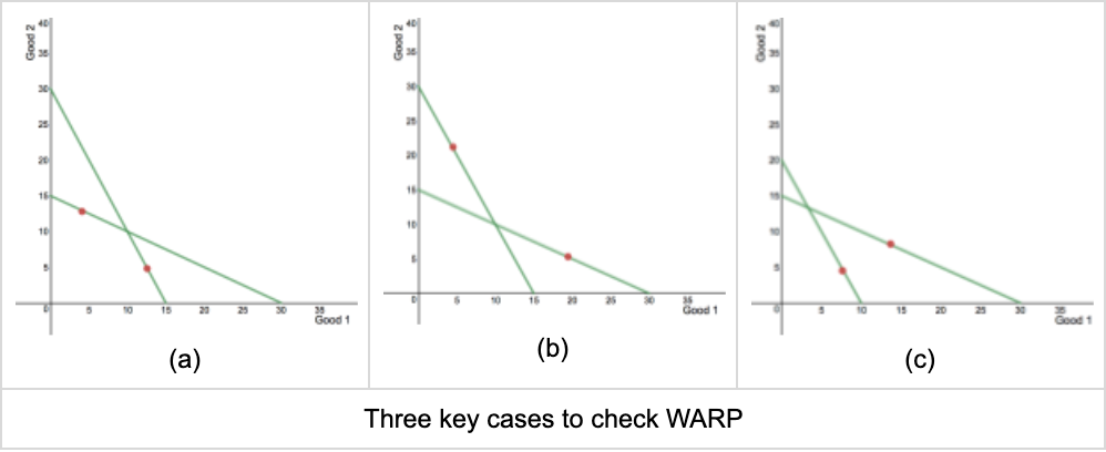
Weak Axiom of Revealed Preference (WARP): Suppose that $(x_1,x_2)$ is selected when the prices are $(p_1,p_2)$, and $(x_1^{\prime}, x_2^{\prime})$ is chosen when the prices are $(p_1^\prime , p_2^\prime)$.

If $p_1x_1^\prime +p_2x_2^\prime \leq p_1x_1+p_2x_2$, then it must be that $p_1^\prime x_1+p_2^\prime x_2 >p_1^\prime x_1^\prime +p_2^\prime x_2^\prime.$

In words, WARP is telling us that if $(x_1,x_2)$ was selected when $(x_1^\prime ,x_2^\prime)$ was affordable, then it cannot be the case that $(x_1,x_2)$ was affordable when the consumer selected $(x_1^\prime , x_2^\prime)$.

The next figure displays the three key cases to check whether WARP is satisfied or not. Using our previous definition, it is easy to see that the only violation happens in panel (a).

Echenique et. al (2010) uses US data for purchasing decisions in the supermarket to check whether people behave according to our model. While they find some violations, they prove that they are not that severe. They also relate the strength of the violations with people’s characteristics. Among other results, they find that older people behave closer to the model.

Market Demand Function

We just learned that the individual demand function of good $i$, with $i=1,2,$ represents the choice of good $i$ in the bundle that maximizes the utility of the consumer for each pair of prices and income level. If we refer to an arbitrary consumer as consumer $j$, then

\[x_1^j (p_1,p_2,m^j) \quad and \quad x_2^j=x_2(p_1,p_2,m^j)\]

indicate consumer $j's$ demands for goods 1 and 2, respectively.

The market demands for these goods are given by

$Q_1^d (p_1,p_2,m^1,m^2,...,m^J)= \sum_{j=1}^{J} x_1^j (p_1,p_2,m^j)$
$Q_2^d (p_1,p_2,m^1,m^2,...,m^J)= \sum_{j=1}^{J} x_2^j (p_1,p_2,m^j)$

where $J$ indicates the number of consumers in the economy. That is, for each fixed vector of prices and income levels, the market demand of each good is simply the sum of the individual market demands of all consumers in the economy for that specific good.

Notice that the market demand of each good depends on the prices of the two goods as well as the income distribution.

We just derived the quantity demanded for each good as a function of the market prices. It is sometimes convenient to express market prices as functions of quantities. We refer to $P(x)$ as the inverse demand function of a certain good.

Example : Suppose that the economy consists of two individuals with demand functions given by

\[x^1(p,m^1)= 20-p \quad and \quad x^2(p,m^2)= 30-3p\]

The aggregate demand function is thereby given by

$Q^d(p,m^1,m^2) = x^1(p,m^1)+x^2(p,m^1)=50-4p \quad if \quad p \leq 10$
$Q^d(p,m^1,m^2) = x^1(p,m^1)+x^2(p,m^1)=20-p \quad if \quad p > 10$

Note that we add quantities for the same price! The next picture illustrates this result.

When demands are linear, then there is usually a kink in the market demand.

In this example, the inverse demand function is given by

$p(Q,m^1,m^2)=12.5-¼Q \quad if \quad Q \geq 10$
$p(Q,m^1,m^2)=20-Q \quad if \quad Q<10$ ■

Let $Q^d (p)$ be the demand function. The elasticity of demand is given by

\[\epsilon =[\partial Q^d (p)/\partial p][p/Q^d (p)]\]

Since, generally, $\partial Q^d (p)/\partial p \leq 0$ , we often express $\epsilon$ in absolute values. The elasticity of demand measures how sensitive is the demand function to price changes.

When $\lvert \epsilon \rvert >1$, we say the demand is elastic. This means that the quantity demanded is very responsive to price changes. It usually happens when the good we are considering has close substitutes. For example, A4 paper from Office World and A4 paper from Boise.

When $\lvert \epsilon \rvert <1$, we say the demand is inelastic. This means that the quantity demanded does not respond very much to changes in prices. It usually happens when the good does not have close substitutes. For example, some medications, like Triluma.

Example : Let $Q^d(p)=a-bp$. The elasticity of demand is

\[\lvert \epsilon \rvert=bp/(a-bp)\]

The next picture shows the way in which $\lvert \epsilon \rvert$ varies with $x$.

Price elasticity with a linear demand: $Q = 20 - p$.

Notice that the good is elastic or inelastic according to the amount that the consumer gets. ■

2.3 Intertemporal Choice

Consuming Today or Tomorrow?

The model we studied in the last section assumes that either there is a single period of time or that the consumer spends all his income every period, without saving or borrowing. This section shows that a similar approach can be used to model consumer behavior across different periods of time.

This extension will allow us to understand the relationship between saving (or borrowing) and the interest rate. It is also important as it shows that, with small modifications, our initial model can accommodate many situations of interest.

In our simple intertemporal choice model, consumers decide how to allocate their income between consumption today and tomorrow. The main components of the model are as follows.

Two goods: current consumption $(c_1)$ and future consumption $(c_2)$
Prices of current and future consumption is 1 (i.e., we assume no inflation)
Income levels: current income $(m_1)$ and future income $(m_2)$
Interest rate: $r$

As you can see, we make a few simplifying assumptions. First, we assume that there is no inflation. Second, we assume there is a bank that allows the consumer to either save his current income $(m_1)$ or to borrow up from his future income $(m_2)$. Moreover, we suppose that the interest rate $r$ is the same for saving and borrowing money. All these restrictions can be easily relaxed with small, though probably tedious, modifications of our main results.

In the intertemporal model, consumers’ preferences are captured by a utility function over current and future consumption

\[u(c_1,c_2)\]

Because we are allowing the consumer to either save or borrow money, the consumer faces a single budget constraint for the “whole life” —or two periods. Expressed in future value, the lifetime income of this person is $(1+r)m_1+m_2$. To understand better this equation, notice that (1+r) represents the extra income the consumer could get in the second period per dollar that he saves in the first period of time. If in period of time 1 the consumer puts 1 dollar of his income in the bank, then in the second period the bank gives the consumer the dollar he invested plus the interest rate r. Similarly, her lifetime consumption (in period of time 2) is $(1+r)c_1+c_2$. His budget constraint simply reflects that these two amounts must be the same. That is,

\[(1+r)c_1+c_2=(1+r)m_1+m_2\]

Notice that, in a graph where $c_1$ is in the horizontal axis and $c_2$ is in the vertical axis, the slope of the budget line is $-(1+r)$.

We can also write the budget line in present value terms

\[c_1+c_2/(1+r)=m_1+m_2/(1+r)\]

In this representation, $1/(1+r)$ indicates the extra consumption the consumer could have in period of time 1 if he sacrifices $1 of consumption in the second period of time. To achieve this goal, the consumer borrows $1/(1+r)$ dollars from the bank in the first period of time with the promise of paying $[1/(1+r)]* (1+r)=1$ to the bank in period of time 2.

The (intertemporal) problem of the consumer is as follows:

\[max_{c_1,c_2} \{u(c_1,c_2): (1+r)c_1+c_2=(1+r)m_1+m_2\}\]

Notice that, from a mathematical perspective, this problem is very similar to our initial consumer choice model! Moreover, it is indeed identical if we let

$x_1=c_1$ and $x_2=c_2$
$p_1=1+r$ and $p_2=1$
($1+r)m_1+m_2=1$

Example : As we just described, we assume no inflation and indicate by $m_1$, $m_2$, and $r$ the corresponding income levels and interest rate. In this example, we will also suppose the consumer has the following utility specification for consumption in periods 1 and 2

\[u(c_1,c_2)=(c_1)^{1/4} (c_2)^{3/4}\]

The problem of the consumer is

\[max_{c_1,c_2} \{(c_1)^{1/4} (c_2)^{3/4}: (1+r)c_1+c_2=(1+r)m_1+m_2\}\]

Given the connection we just established between this model and the initial consumer problem, we can use our previous results to state that

$c_1^* =(1/4)[(1+r)m_1+m_2][1/(1+r)] \quad and \quad c_2^* =(3/4)[(1+r)m_1+m_2] \quad$ ■

Investment Decision

We just studied the optimal allocation of consumption levels between today and tomorrow. Let us next assume that our intertemporal consumer faces the possibility of investing some amount of money today with the promise of receiving some specific return tomorrow. Should the consumer make such an investment? We now develop a criterion which the consumer should use in deciding whether or not to do so.

To be more clear, let us consider an investment which has a negative cash flow of -$A today —the investment— and a positive cash flow of $B in 1 year —the return. The question we want to address is

\[Should \;the\; person\; invest\; in\; this\; project?\]

The answer to this question is indeed very simple.

The person should invest if (and only if)

\[-A + B/(1+r) \geq 0\]

(Positive Net Present Value in Finance.) The reason is that if $-A + B/(1+r) \geq 0$, then the budget line of the consumer shifts up.

Notice that the previous rule does not depend on the preferences of the consumer!

2.4 Choice Under Risk

In this section, we study individual behavior with respect to choices involving risk. We face risks in almost every single decision we make since, in most cases, it is hard to anticipate the exact consequences of each alternative.

Let’s start with an example. As an economics professor at UC Berkeley, Gary Becker had to give an exam at 8:00 AM. He arrived at the university at 7:55 AM, so he did not have enough time to go to the parking lot and be on time for the test. He faced two options:

go to the parking lot, so to avoid the parking ticket, but be late for the exam with certainty; or
park in front of the Economics Department, so to be on time for the exam, but face the risk of getting a parking ticket.

As you can see, each option has pros and cons. The question is how to compare them! To do so we need a model that would allow us to compare options in which we are not sure about the final outcomes. We next present the most commonly used method.

In economics, we typically use the framework of Expected Utility (EU). In this approach, every possible outcome has a utility level associated with it. In this example, $u(late, no penalty)$ would denote the utility that Gary Becker gets from option (1). Under option (2), there are two possibilities, he either gets caught or he doesn’t. Let $u(on time, penalty)$ and $u(on time, no penalty)$ indicate the utility levels under these two possible outcomes of option (2). Also, suppose that he estimates that if he parks in front of the Economics Department, then the probability of getting caught is $p$. According to the expected utility approach, Gary Becker values the risky alternative as a weighted combination of the utilities he could experience in that course of action. Following that logic he should decide to be late if and only if:

\[u(late, no penalty)>(p)u(on time, penalty)+(1-p)u(on time, no penalty)\]

Otherwise, he should choose to “break the law”, and park in front of the Econ Department³.

More generally, the expected utility model assumes that the utility a person gets from each risky choice depends on (i) the utility of the different outcomes the individual might face; and (ii) the probability of each of these possible outcomes. In particular, the valuation of a risky choice in the expected utility model is as follows:

\[EU = p_1 u(c_1) + p_2 u(c_2)\]

where $c_1$ and $c_2$ are two possible outcomes usually measured in monetary terms (for example $1 and $10), and $p-1$ and $p-2$ are their corresponding probabilities (for example $⅓$ and $⅔$, respectively). Under this specification, the overall utility is just the weighted average of the utility that the person gets under each possible circumstance, where the weights are the probabilities that the person assigns to the different events.

As we mentioned earlier, though the expected utility approach is probably the most widely utilized method, it is not the only model that has been used to study choice under risk. The field of behavioral economics studies other conceptual approaches, among which the prospect theory by Tversky and Kahneman (1979) is probably the most prominent one.

In what follows, we will only consider situations where the different outcomes of the risky choice are simply different amounts of money. In that sense, we will restrict attention to situations that are similar to the ones that consumers face when they buy lottery tickets or go to the casino.

Example : (Lottery) An individual has $100 in his wallet and is evaluating whether to buy a lottery ticket. The ticket costs $20 and he knows that with 50% chance he can get $40, and with 50% chance he gets $0. In our notation, $c_1=100-20+40=120, c_2=100-20=80, p_1=0.5$ and $p_2=0.5$. Let us also assume, the utility function of this person is given by:

\[u(c_i)=c_i^{1/2}\]

where $c_i$ is the money that the consumer gets in each outcome $i$. Under this specification, if the person buys the ticket, his expected utility (denoted by EU) is given by:

\[Expected \; Utility \; of \; the \; Lottery \;Ticket \;(EU) = \frac{1}{2} u(100-20-40) + \frac{1}{2} u(100-20)\] \[\qquad \qquad \qquad \quad = \frac{1}{2} (120)^{1/2}+ \frac{1}{2}(80)^{1/2}\] \[\qquad \qquad \qquad \qquad = 9.95 \qquad \qquad \qquad \quad\]

On the other hand, if the individual does not get the ticket, his utility is $u(100)=(100)^{1/2}=10$, with certainty. Since $10 > 9.95$, this consumer will rather prefer not to buy the ticket for the lottery. ■

It is important to notice that the expected value of buying the ticket in the previous example is

\[\frac{1}{2}(100-20+40) + \frac{1}{2}(100-20) = 100\]

That is, it is the same as not buying the ticket. Yet, this consumer preferred to avoid taking the risk involved in the lottery. The next example shows the key role that the shape of the utility function has in determining whether a person takes or not a specific risk.

Example : (Investment) An individual is contemplating the possibility of either investing his money in a risky project that pays $36 if he wins and $0 otherwise or in a safe project that always pays $18. He estimates that the probability of winning in the risky project is ½. That is,

\[c_1=36, \, c_2=0, \, p_1=0.5 \quad and \quad p_2=0.5\]

We are interested in a simple question: Should a rational person invest in the risky project?

We next show that the answer of this question depends on the preferences of the individual, which are captured by the shape of the utility function u.

If the person gets involved in the risky project, then his expected utility is

\[EU[risky \; project]=\frac{1}{2}u(36)+\frac{1}{2}u(0)\]

Since the safe option always pays $18, he should invest in the risky project whenever

\[EU[risky \;project]=\frac{1}{2}u(36)+\frac{1}{2}u(0) \geq u(18)\]

Otherwise, this person would be better off putting his money in the safe option.

Without any other information regarding the shape of u, we cannot answer our initial question. We next contemplate three different possibilities.

Let us assume first that $u(c_i)=(c_i)^{1/2}$. In this case, the expected utility of the risky project is

\[EU[risky \;project]=\frac{1}{2}u(36)+\frac{1}{2}u(0)=\frac{1}{2}(36)^{1/2}+\frac{1}{2}(0)^{1/2} = 3\]

In addition, the utility he gets from the safe project is $(18)^{1/2} \approx 4.24$. Since

\[EU[risky \;project]=\frac{1}{2}(36)^{1/2}+\frac{1}{2}(0)^{1/2} = 3 <4.24\]

we conclude that this person should select the safe option. The following picture illustrates this first situation.

Risk averse choice

Note: You can access an interactive version of this graph here.

Let us now suppose that $u(c_i)=c_i$. In this case, we have that

\[EU[risky \;project]=\frac{1}{2}u(36)+\frac{1}{2}u(0) =\frac{1}{2}(36)+\frac{1}{2}(0)=18\]

In addition, the utility from the safe project is $u(18)=18$. Thus, this person is just indifferent between the safe and the risky option.

Risk neutral choice

Finally, let us set $u(c_i)=(c_i)^2$. In this case, we have that

\[EU[risky \;project]=\frac{1}{2}u(36)+\frac{1}{2}u(0) =\frac{1}{2}(36)^2+\frac{1}{2}(0)^2=648\]

In addition, the utility from the safe project is $u(18)=(18)^2=324$. Thus, this person clearly prefers the risky investment. ■

Risk loving choice

We often classify individuals according to their attitudes toward risk. As we shall see, the standard classification is intimately related to our last example. It involves the comparison between the expected utility of the risky project

\[p_1 u(c_1)+ p_2 u(c_2)\]

and the utility of the person evaluated at the expected value of the risky project

\[u(p_1c_1+p_2c_2)\]

The expected value of the risky project —$p_1c_1+p_2c_2$—- can be thought of as the amount of money that a person who invests in the risky project many times would get on average.

The next table classifies people according to attitudes toward risk and establishes a connection between these attitudes and the curvature of the utility function.

Attitude/Behavior	Shape of utility function	Property of utility function
Risk Averse	Concave Utility	$p_1 u(c_1)+p_2 u(c_2)<u(p_1c_1+p_2c_2)$
Risk Neutral	Linear Utility	$p_1 u(c_1)+p_2 u(c_2)=u(p_1c_1+p_2c_2)$
Risk Loving	Convex Utility	$p_1 u(c_1)+p_2 u(c_2)>u(p_1c_1+p_2c_2)$

Example : Suppose that, as in the last example, an individual is contemplating the possibility of either investing his money in a risky project that pays $36 if he wins and $0 otherwise or in a safe project that always pays $18. The probability of winning in the risky project is again 1/2.

In the previous example we studied the investment decision of three individuals that differed regarding the shape of the utility function: (i) $u(c_i)=(c_i)^{1/2}$; (ii) $u(c_i)=c_i$; and (iii) $u(c_i)=(c_i)^2$. We found that the first individual would not invest, the second one was indifferent, and the third one would always invest in the risky project. Given our last table, we could have made the prediction without any calculation!

The reason is that the expected value of the risky project was given by

\[\frac{1}{2} 36 + \frac{1}{2} 0 = 18\]

This is the same as the money the individual makes with the safe investment. In addition, $u(c_i)=(c_i)^{1/2}$ is a concave function, $u(c_i)=c_i$ is a linear function, and $u(c_i)=(c_i)^2$ is a convex function. ■

To do so, we also require the preferences to be continuous. Roughly speaking, “preferences are continuous” if whenever an alternative A is preferred to an alternative B, any option A’ that is sufficiently similar to option A is also preferred to option B. ↩
Notice that we have chosen to draw only four out of an infinite number of possible indifference curves. ↩
This example is given by Gary Becker as the starting point of his economic analysis of criminal decisions. ↩

Price of good 1	Price of good 2	Income	Choice of good 1	Choice of good 2
\(p_1\) = 2	\(p_2 = 1\)	\(m=10\)	\(x_1^* = 4\)	\(x_2^* = 2\)
\(p_1\) = 1	\(p_2 = 1\)	\(m=8\)	\(x_1^* = 1\)	\(x_2^* = 7\)

Utility Function	Mathematical Form
Perfect Substitutes	\(u(x_1,x_2) = ax_1 + bx_2\)
Perfect Complements	\(u(x_1,x_2) = min\{ \frac{x_1}{a} , \frac{x_2}{b} \}\)
Cobb-Douglas	\(u(x_1,x_2) = (x_1)^a (x_2)^b\)
CES	\(u(x_1,x_2) = (ax_1^r + bx_2^r)^{1/r}\)

Attitude/Behavior	Shape of utility function	Property of utility function
Risk Averse	Concave Utility	\(p_1 u(c_1)+p_2 u(c_2)<u(p_1c_1+p_2c_2)\)
Risk Neutral	Linear Utility	\(p_1 u(c_1)+p_2 u(c_2)=u(p_1c_1+p_2c_2)\)
Risk Loving	Convex Utility	\(p_1 u(c_1)+p_2 u(c_2)>u(p_1c_1+p_2c_2)\)

Bundle	Utility 1	Utility 2	Utility 3
\((16,1)\)	8	12	4
\((3,3)\)	7	9	2
\((2,4)\)	6	9	2
\((2,2)\)	3	2	-1